Geospatial · Remote Sensing · 2026
Denver Urban Tree Classification: Mapping a Neighborhood's Canopy from Free Imagery
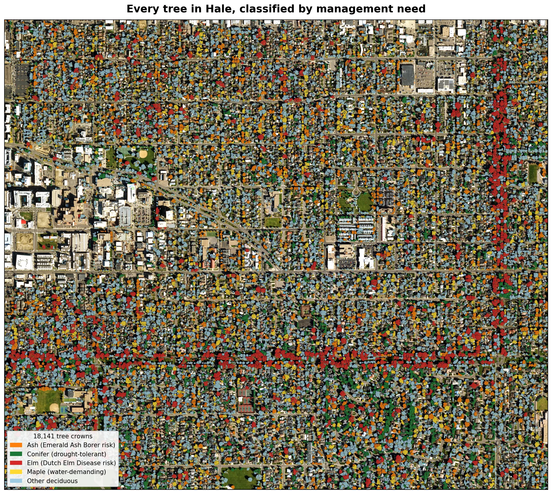
Denver's foresters manage tens of thousands of street and park trees with a small crew, and the first thing they need is a map of what is growing where. I wanted to see how much of that map I could build from free public imagery, without sending anyone into the field to identify trees one at a time. The answer came in two halves. Telling one species from another this way works for some species but not reliably enough to replace a survey, because too many species reflect light in almost the same way. But sorting trees into the few groups a forester treats differently works well enough to be useful. This project is that second map: every tree crown in Denver's Hale neighborhood, sorted into five management classes from aerial imagery, a satellite time series, and airborne laser scanning.
The project grew out of a short course on applying machine learning to environmental satellite data, run by the American Meteorological Society with NASA and CIRA. Two of its sessions set the direction, one on machine learning for land-cover classification and one tracing the field from random forests to foundation models, and that span became the shape of the work below, from a gradient-boosted classifier to the foundation models tested at the end.
Tom Shanks
- Overall accuracy
- 69.0%
- Spatially validated
- ~66%
- Over pixel baseline
- +30.7 pts
- Crowns mapped
- 18,272
Why species is the wrong target
The first instinct is to classify each tree by species, so I tried it. With a simple pixel-by-pixel approach across ten common species the accuracy sat near 17 percent, barely above guessing. NAIP, the US Department of Agriculture's aerial photography, carries only four color bands (red, green, blue, and near-infrared), and at the level of single pixels many species reflect those four bands almost identically. The fuller crown model built below recovers a good deal more of the species signal, as I come back to later, but for what a city actually does the species label is still not the target worth chasing.
I changed the question to match what the data can support and what a forester actually needs. Crews are not dispatched by Latin name. They act on a few practical categories: ash at risk from the Emerald Ash Borer, elm at risk from Dutch Elm Disease, water-demanding maples, drought-tolerant conifers, and everything else. Collapsing ten species into those five management classes turns a problem the imagery cannot solve into one it can.
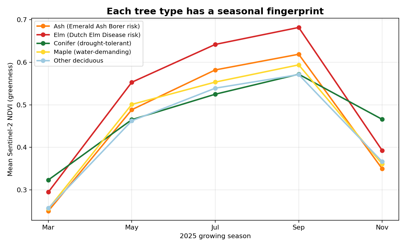
The classes also separate over the seasons, which a single photograph cannot capture but a satellite that revisits the same spot can. I built a five-date series from Sentinel-2, the European Space Agency's free satellite, across the 2025 growing season and measured greenness with NDVI (a standard index where higher values mean more living leaf). Each class moves through the year a little differently. Conifers hold their color into November while the deciduous classes leaf out and fade, and that motion gives the model a signal a midsummer snapshot would miss.
Building the map
To classify a tree I first have to find it. Instead of labeling individual pixels I delineated whole tree crowns, which keeps each tree as one object and follows how Cross (2019) approached tree mapping in Costa Rican forest. The crowns come from a canopy height model, a raster of how tall the vegetation stands, built from DRCOG's 2020 airborne LiDAR (laser scanning that measures height directly). A watershed segmentation, masked to vegetation, split the canopy into 18,272 individual crowns.
For each crown I measured 109 features: color and near-infrared statistics from NAIP, the five-date Sentinel-2 series and its seasonal changes, several vegetation indices including the red-edge and water indices Cross found most useful for separating species, and height and shape from the LiDAR. I attached a known species to a crown wherever it fell within three meters of a tree in the city's arborist inventory, which gave 3,764 labeled crowns to learn from. I compared four classifiers by cross-validation, and a gradient-boosted model came out ahead.

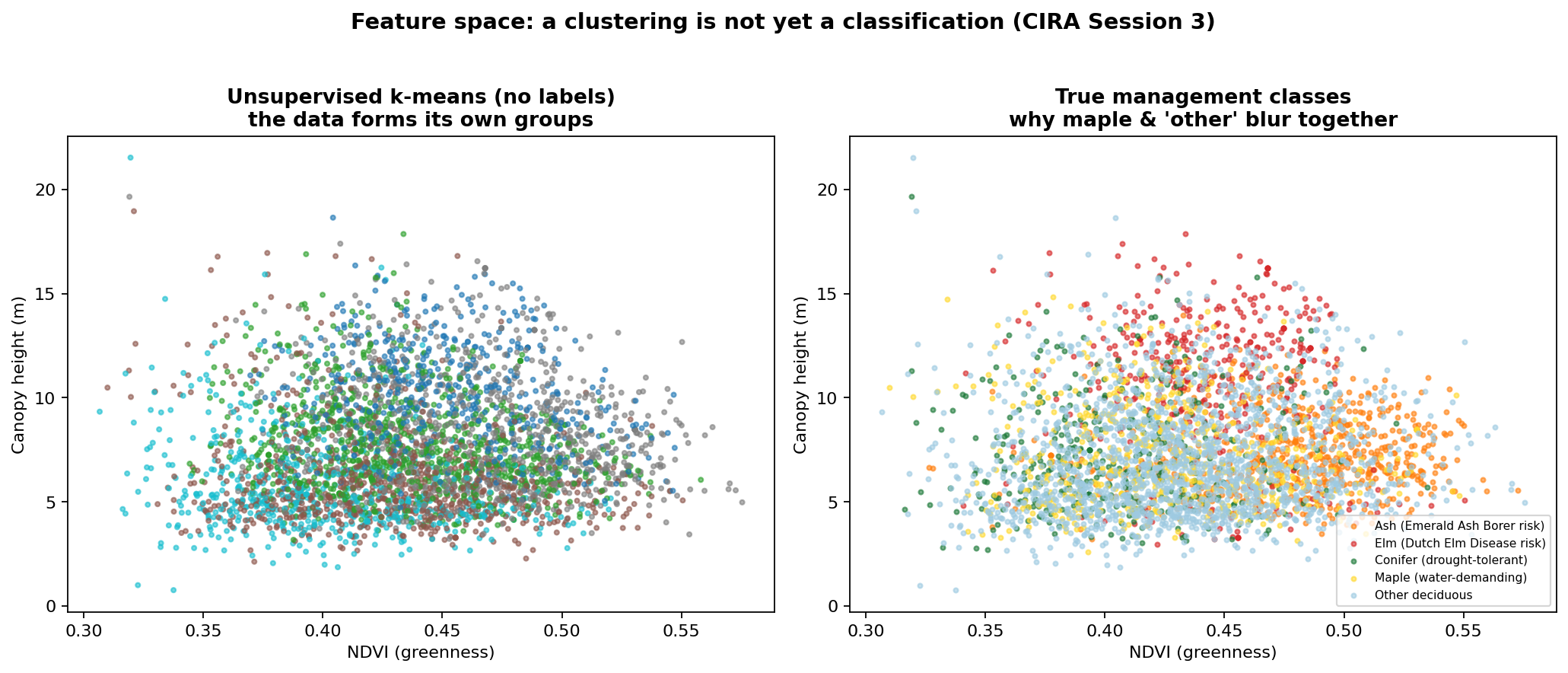
A look without labels
Before trusting a trained model it helps to see whether the trees group on their own. Plotting every crown by greenness and height and letting a clustering algorithm sort them, with no labels at all, shows real structure in the data. It also shows why the job is hard. When I color the same plot by the true management classes, maple sits almost on top of the catch-all deciduous group, which is exactly where the trained model later makes most of its mistakes.
Results
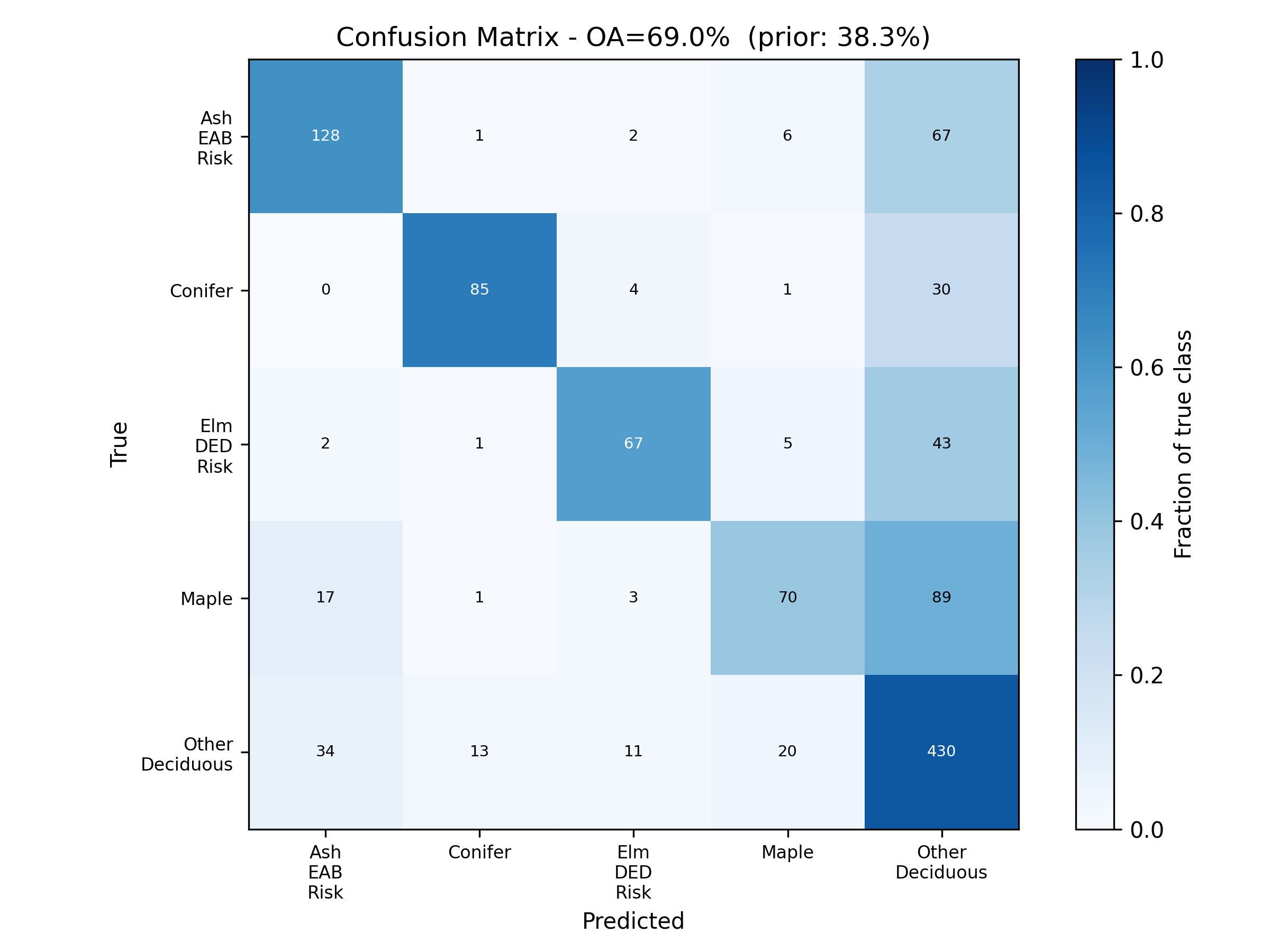
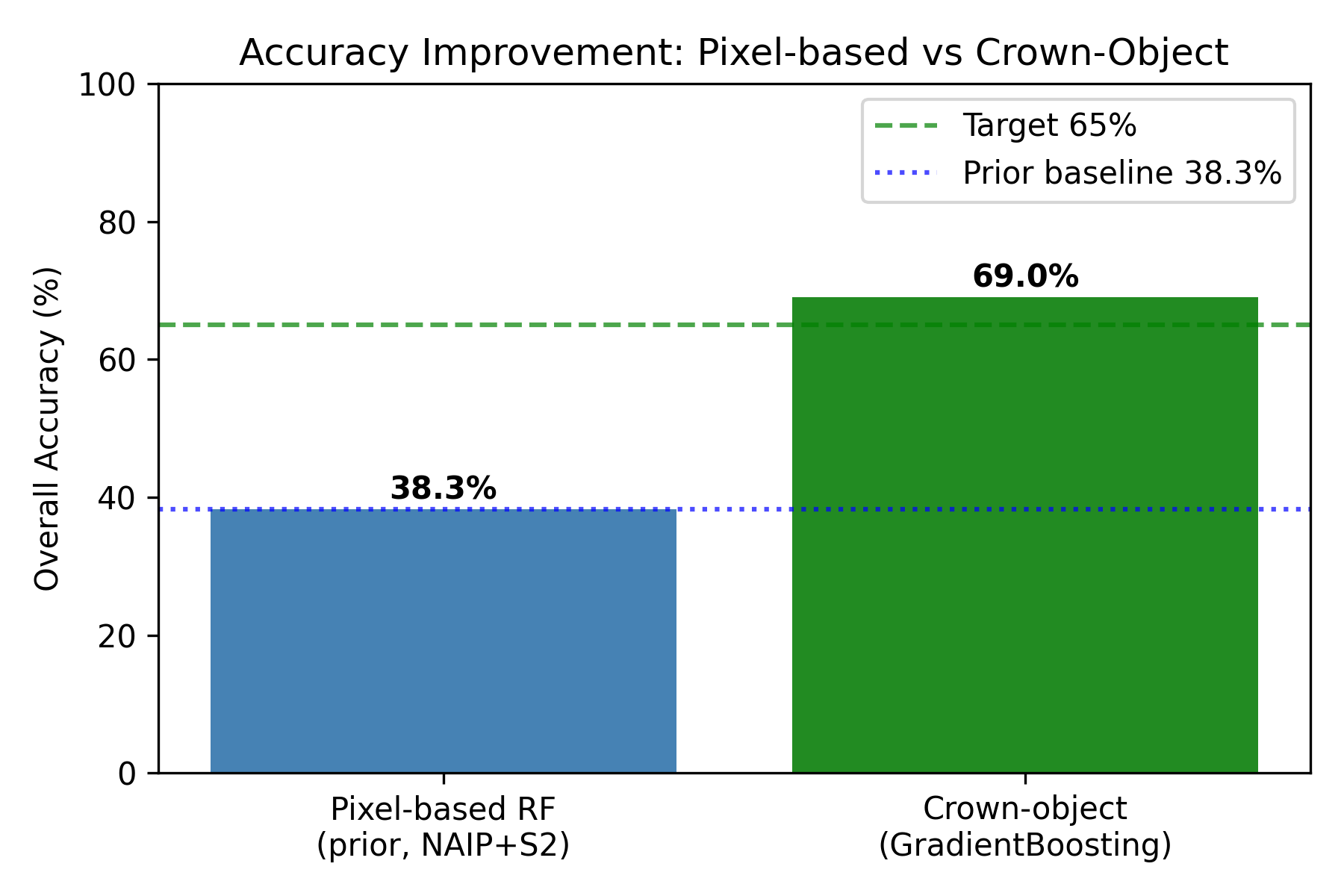
The model reaches 69.0 percent overall accuracy across the five classes, up from 38.3 percent for an earlier version that worked pixel by pixel, a gain of about 31 points. Balanced accuracy, which averages the per-class scores so the large groups do not dominate, is 62.8 percent. The classes a forester cares most about score highest. Conifers and ash are recovered well, while maple is the weakest because it shares so much spectral and structural ground with the other deciduous trees.
| Management class | Precision | Recall | F1 | Crowns |
|---|---|---|---|---|
| Ash (Emerald Ash Borer risk) | 0.71 | 0.63 | 0.66 | 204 |
| Conifer (drought tolerant) | 0.84 | 0.71 | 0.77 | 120 |
| Elm (Dutch Elm Disease risk) | 0.77 | 0.57 | 0.65 | 118 |
| Maple (water demanding) | 0.69 | 0.39 | 0.50 | 180 |
| Other deciduous | 0.65 | 0.85 | 0.74 | 508 |
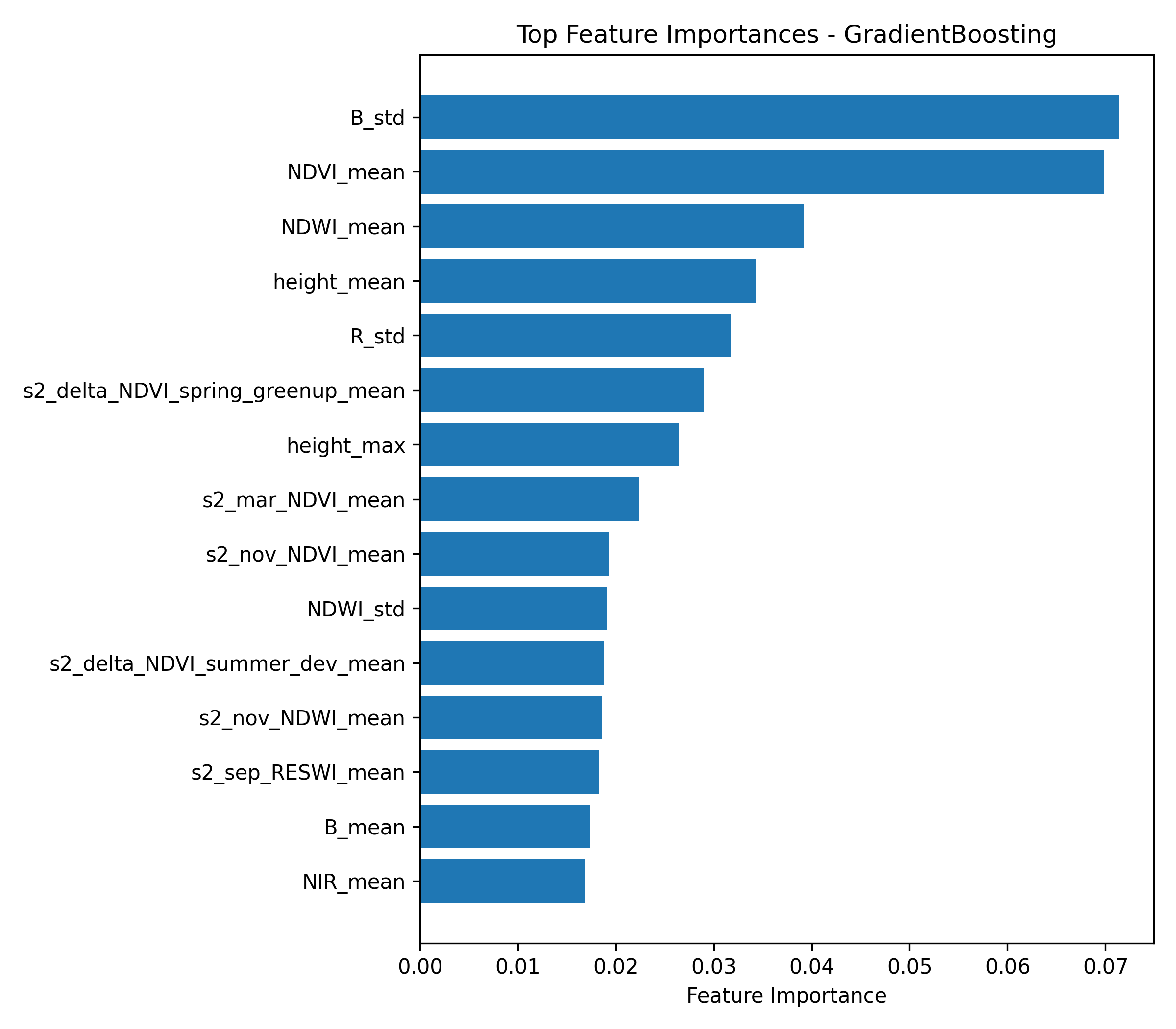
The model leans most on color and season rather than on structure. The Sentinel-2 time series and the NAIP bands together carry close to nine tenths of the decision, and the LiDAR height about a tenth. So the result is mostly a question of reflectance, of how each canopy reflects light across the bands and across the year. That is the same premise Cross relied on with commercial satellite imagery in Costa Rica, carried here to free public data and to an urban canopy.
How honest is that number
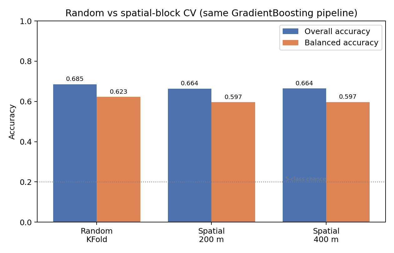
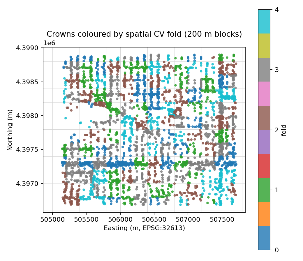
A single accuracy number from a random split tends to flatter a map like this. Neighbouring crowns are photographed under the same light and often belong to the same planting, so if some land in training and their neighbours in the test set, the model can look better than it really is. To get an honest figure I held out whole spatial blocks at a time, 200 and 400 meters across, so entire stretches of the neighborhood stayed out of training together.
Under that stricter test the accuracy settles around 66 percent, roughly two points below the random-split figure and steady across block sizes. The small gap tells me the map generalizes across the neighborhood rather than memorizing it. The one class that slips is maple, for the same reason it was weakest to begin with. This follows a habit from NASA and NOAA's remote-sensing training: give the model an honest grade, and do not assume a model trained on one place transfers to another.
| Evaluation | Overall accuracy | Balanced accuracy |
|---|---|---|
| Random split, same model | 0.685 | 0.623 |
| Spatial blocks, 200 m | 0.664 | 0.597 |
| Spatial blocks, 400 m | 0.664 | 0.597 |
How far species can go
Having built the model, I went back to the harder question and asked it to name the species directly. Across the twenty-one species with enough labeled trees to learn from, it was right about fifty-four percent of the time. That is a long way past the seventeen percent a pixel-based approach managed, and far above the roughly five percent of pure guessing. The distinctive species come back well, blue spruce, American elm, honeylocust and ash among them, while the look-alikes blur, the lindens with each other and the oaks and ornamental maples into the broadleaf crowd.
So species is not hopeless from free imagery once you work crown by crown rather than pixel by pixel. It is simply not reliable enough to stand in for a field survey, and a city does not need it to be. The five management classes stay the headline because they are what a crew acts on, but the species result shows how much signal the crown approach pulls out of the same free data.
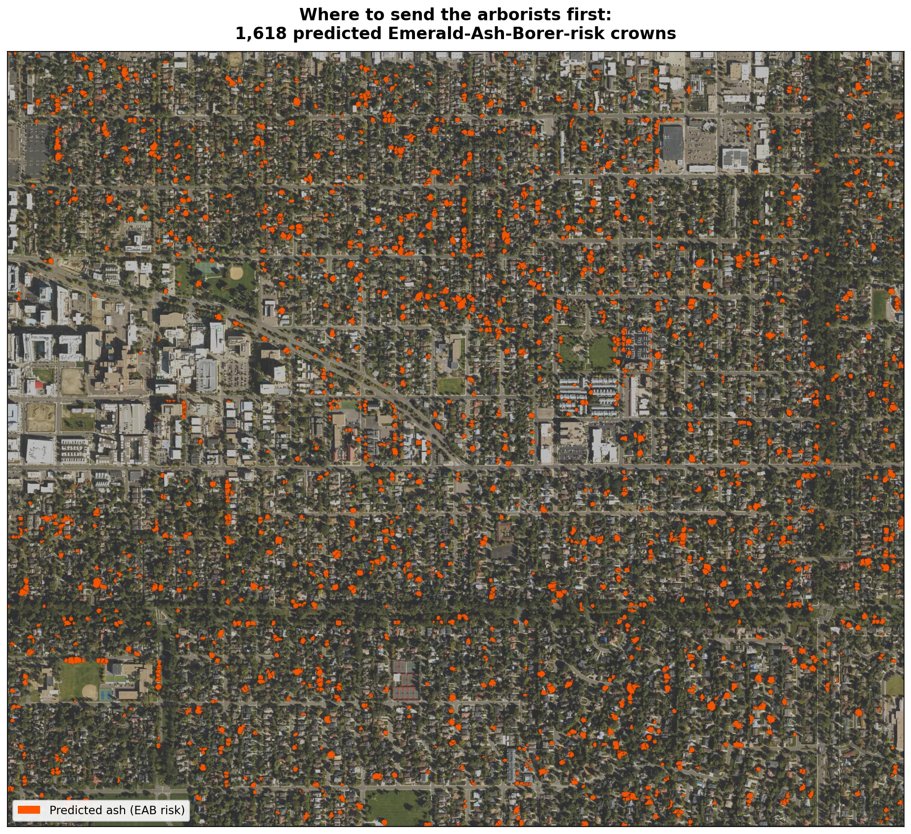
From map to action
The accuracy figure matters less than the work the map saves. The Emerald Ash Borer kills untreated ash and is moving through the Front Range, and a crew can only inspect so many trees in a season. The most useful thing the model produces is a short, ranked list of where the ash most likely are, so the first trucks go to the right blocks. About sixteen hundred crowns are flagged as likely ash for a crew to confirm and treat. It points the field work rather than replacing it. In a later test, adding an October image, when ash turns color on its own schedule, improved how reliably the model finds ash by about seven points, the single most useful addition for this borer-triage job.
Watching the canopy change over time
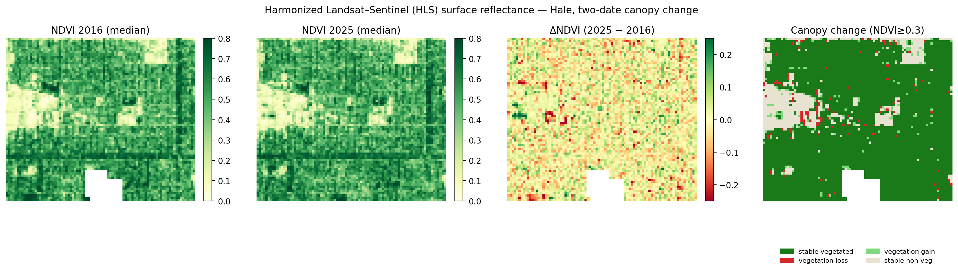
The crown map is a single snapshot. To watch the canopy change I needed a second date and a sensor that revisits often, so I turned to the Harmonized Landsat-Sentinel product, or HLS, a free NASA dataset that puts the Landsat and Sentinel-2 satellites on one 30 meter grid and delivers calibrated surface reflectance every few days. Surface reflectance is the analysis-ready standard the training I took emphasized, and it is the one thing the crown model above does not use, since that model still learns from raw NAIP brightness values while HLS measures light corrected to the ground.
I built a cloud-free summer composite of Hale for 2016 and for 2025, measured greenness in each, and compared them. The neighborhood canopy turned out to be broadly stable. Average greenness barely moved, and the patches that grew greener and browner roughly cancel, with about two percent of the area losing vegetation and two and a half percent gaining it. I am careful not to over-read the rest, because two summer snapshots a few years apart differ a little just from sun angle and the exact day they were captured, so the stable picture is the trustworthy part rather than the sign of every small change.
The trade is resolution. At 30 meters a single HLS pixel covers several trees plus the street and yards around them, so HLS cannot pick out one crown the way the 1 meter model does. The two work together. The crown model says what each tree is, and HLS says how the whole neighborhood's greenness is holding up over time.
Where the field is going: a foundation model
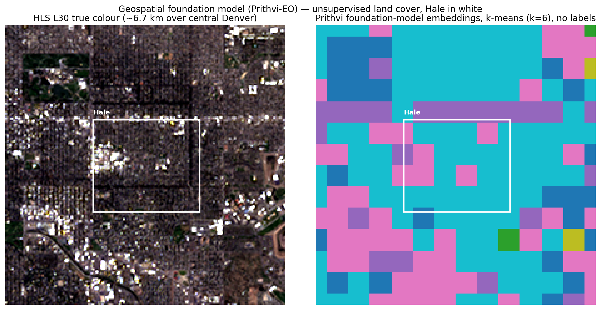
The newest approach in this field does not hand-build features at all. Geospatial foundation models are large neural networks pretrained on enormous amounts of satellite imagery, much as a language model is pretrained on text, and the same pretrained model can then be reused for many tasks. To see where my project sits next to that frontier, I ran Prithvi, a foundation model from NASA and IBM trained on Harmonized Landsat-Sentinel imagery, over central Denver. I handed it a six-band HLS image and, with no labels, let it turn the scene into its own learned features, then grouped those into land-cover types.
What comes back is honest about the promise and the limit at once. The model organizes the scene on its own, but Prithvi reads the image in roughly 480 meter patches, so it sees central Denver as a largely uniform residential canopy with only coarse distinctions. That is the same lesson from a new direction. The variation that matters for urban forestry lives at the scale of a single tree, which is exactly where my one meter crown model works, and where a foundation model would need fine-tuning on a graphics card to follow. I include it as a marker of the road ahead, and because the project now spans the full range the field uses, from a random forest to a foundation model.
Learned models at the crown scale
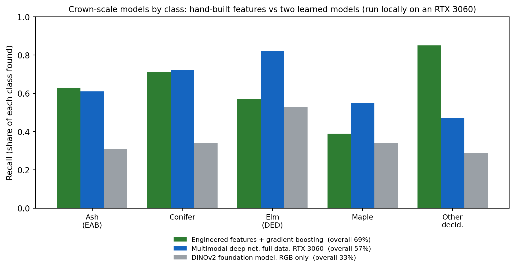
The newest approach lets a model learn its own features instead of using hand-built ones, so I tried that at the scale this project works at, one tree at a time, on a graphics card here at my desk. I started with the simplest version, a general vision foundation model called DINOv2, and gave it a small aerial chip of each tree. With only the red, green and blue of a single photo to work from it reached about a third of the crowns, far behind the engineered model.
Then I built a model that sees everything the engineered features see: a small network that takes the near-infrared and the laser-measured height alongside the color image and reads the six-date Sentinel-2 series for how each tree changes through the year. That closed almost all of the gap. It matched the engineered model on balanced accuracy, the figure that weights every class equally, and it was the better of the two on the hardest disease classes, lifting elm recall from 0.57 to 0.82 and maple from 0.39 to 0.55. It came in lower on overall accuracy, because it gives up some of the large catch-all class to do better on the rare ones.
The pattern across the three models is the honest lesson of the whole project. A model is only as good as the data it is shown. The general model with color alone trails badly, the same idea fed the full multispectral, seasonal and height data pulls level with years of hand-built features, and the gradient boosting still edges ahead on the headline number because, with only a few thousand labeled trees, hand-built features are hard to beat outright. That last point is what makes pretraining the real next step.
| Crown-scale model | Overall accuracy | Balanced accuracy |
|---|---|---|
| Engineered features + gradient boosting | 0.690 | 0.628 |
| Multimodal deep net (full data, local GPU) | 0.569 | 0.632 |
| DINOv2 foundation model (RGB only) | 0.329 | 0.360 |
Where this leaves it
The project now runs the full span the field uses, on a single neighborhood and on free data: an object-based crown model that maps management classes and reaches into species, an honest spatial check on what that accuracy really means, a surface-reflectance look at how the canopy changes over time, and a stack of learned models, from two foundation models to a purpose-built deep net, run over the same ground. The real frontier from here, and the step the deep net points straight at, is a foundation model pretrained on exactly the kind of multispectral and seasonal data this problem depends on, at fine resolution, which is a research undertaking rather than a missing afternoon's work.
Data and tools
Every input is free and openly licensed, and the whole pipeline runs from a single script, so the result is reproducible and the dataset is easy to share. The methodology is adapted from Cross (2019), who classified tree species in Costa Rican forest from WorldView-3 satellite imagery. The contribution here is carrying that object-based, reflectance-driven approach to free imagery and to the practical problem of managing an urban canopy.
| Dataset | Source | License |
|---|---|---|
| NAIP 2023 aerial imagery (4 band, 30 cm) | USDA NRCS, via AWS | Public domain |
| Denver tree inventory (arborist survey) | Denver Open Data Portal | CC BY |
| Canopy height model | DRCOG 2020 3DEP airborne LiDAR | Public domain |
| Sentinel-2 surface reflectance, 5 dates | ESA Copernicus | Free, open |
| HLS surface reflectance (L30/S30, 30 m) | NASA LP DAAC, via Earthdata | Free, open |
Built with Python, Rasterio, GeoPandas, scikit-image, scikit-learn and XGBoost, with QGIS for inspection. Study area: the Hale neighborhood, about 4.6 square kilometers.
Source available on request.